


The Sperry Sonar Propagation and Transducer Computer
Originally published in the Slide Rule Gazette, Issue 9, Autumn 2008
Originally published in the Slide Rule Gazette, Issue 9, Autumn 2008
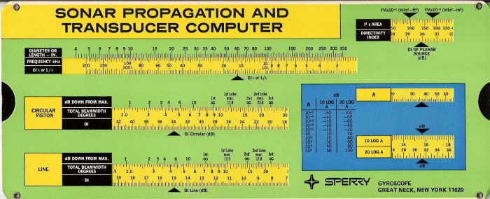
Fig.1. Sonar Propagation and Transducer Computer, side 1, for Transducers and Arrays
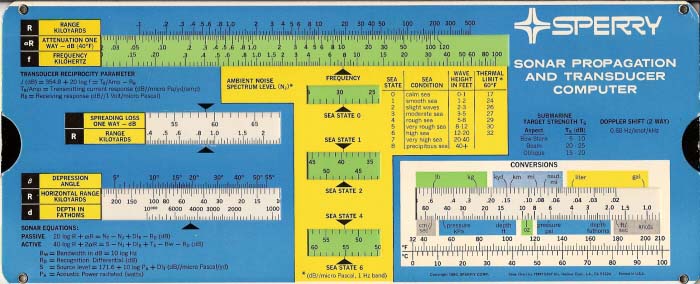
Fig.2. Sonar Propagation and Transducer Computer, side 2, for Sonars
In 1982, the British arm of Sperry Gyroscope was bought by British Aerospace. Sperry Gyroscope had its headquarters and main facilities at Bracknell, Berkshire with a manufacturing facility at Plymouth, and an Underwater Research and Engineering Unit in Weymouth. At that time I was working for British Aerospace at Filton, Bristol as Chief Engineer Underwater Projects and, in 1984, when the Weymouth facility needed a new Chief Engineer and deputy to the director in charge, I was given the job and duly moved to Weymouth. Amongst the projects at Weymouth at that time was a new type of sonar. My previous experience was limited to guided weapons, and torpedo fuel and transmission systems, so I had to learn a bit about sonar pretty quickly. To help me I was given the slide chart, which is the subject of this article.
Before describing the sonar propagation and transducer computer, perhaps I had better say a little about sonar and transducers. Sonars use acoustic waves to locate objects in water, form images of them and determine their range. There are two basic classes of sonar, active and passive. Active sonars transmit pulses of sound, which are reflected from, amongst other things, the intended target. Some of this reflected sound hopefully finds its way back to its source (or sometimes a separate receiver) where it is received and processed. Passive sonars are purely receiving systems, listening for noises from a target amongst all the other noises present in the water. I should perhaps add that I am not using target in the purely military sense but to indicate the feature of interest, which could be a ship, submarine, wreck, underwater pipeline, or even a shoal of fish. Sonar has many uses besides military ones.
Any sonar system consists of three main elements, a transducer array or arrays, a signal processing system to detect signals received by the array, and a data processing system to isolate and record/display the wanted signals (in early systems this was an operator with a set of headphones and possibly a tape recorder). An active system has in addition a signal generator and amplifier to drive the transmitting transducers. So the transducer is a device that converts electrical signals into sound and/or vice versa. Transducers exist in many forms and may be used either singly or in arrays. The latter can take many forms, the chief ones being line, planar and cylindrical. Depending upon their function, sonars operate over a wide variety of frequencies. Generally, long range requires low frequency, which in turn requires large arrays and lots of power (in the case of active systems). Image forming on the other hand requires high frequencies to obtain sufficient resolution.
Any transducer or transducer array has a beam pattern and this is a function of the array size and shape in relation to the operating wavelength, which is proportional to the inverse of frequency. If the array is smaller in size than the wavelength then the beam pattern will be essentially omnidirectional. As the array size increases in relation to the wavelength the main beam will get narrower and narrower; there will be side-lobes but we will ignore these. This directivity is of considerable benefit and is one of the terms in the sonar equation, of which, more later.
The Sonar Propagation and Transducer Computer came in a vinyl wallet with a twelve-page booklet of instructions. It was (still is) the copyright of the Sperry Corporation and was produced for them by Perrygraf in the USA in 1980/1. It is made of stout, plastic faced card and measures 9¾ inches by 4 inches. It is attractively coloured in blue, green and yellow and is mostly clear to read and use. Most of the scales are logarithmic so I suppose it could be classed as a specific purpose slide rule. It is no coincidence that many of the scales are logarithmic since sonar performance is normally calculated and expressed in decibels. The instruction booklet also contains the formulae on which its scales and computation are based and also worked examples but I do not intend to repeat all of those here.
Let us first look at transducer calculations. The computer covers just two types, the circular piston transducer and the line array; however a planar array can be considered as the product of two line arrays and other types of array can be similarly treated. A circular piston transducer is so called because it has a circular radiating face, which moves in and out like a piston. Fig.1 shows the side of the computer, which is used for determining the directivity and beam pattern of transducers and arrays.
The Sonar Propagation and Transducer Computer came in a vinyl wallet with a twelve-
Let us first look at transducer calculations. The computer covers just two types, the circular piston transducer and the line array; however a planar array can be considered as the product of two line arrays and other types of array can be similarly treated. A circular piston transducer is so called because it has a circular radiating face, which moves in and out like a piston. Fig.1 shows the side of the computer, which is used for determining the directivity and beam pattern of transducers and arrays.
The upper left-hand scales are used first. The operating frequency in kHz is set against the array length or, for a single transducer, the transducer diameter. The beamwidth can now be read from the appropriate scale (either the one for a circular piston or the one for a line). However one must first define beamwidth. Typically this will be defined as when the sound level is half the peak value (i.e. 3dB down) but one might also want to know the 10dB down value, or the angle of the first null, or the first side-lobe maximum, etc. Having chosen the definition(s) of interest the total beamwidth or angle for each, in degrees, can be read from the adjacent scale. At the same setting, the directivity index (DI dB) can be read at the arrow on the scale below. The diameter or length to wavelength ratio (D/λ or L/λ) can also be read at the arrow on the scale adjacent to the frequency one that you started with. The scale can also be used to find the wavelength at the operating frequency, assuming a velocity of sound in seawater of 5000 feet per second.
In the top right corner there is a small window for finding the directivity index of a planar source of any shape. The radiating area in square inches or square feet is multiplied by the frequency in kHz, and the resulting value is set against the appropriate arrow. The directivity index (DI dB) can then be read off the scale below against the DI arrow. It should be noted that the directivity and beamwidth scales for planar sources and piston transducers assume that they are baffled, i.e. they only radiate in the forward direction from the surface.
The final part of this side enables conversions to and from decibels. Values of ‘A’ can be converted to 10logA and 20logA, or vice versa.
Let us now look at the other side and propagation calculations (Fig.2). There are two components to the loss of sound in water, spreading, which is just a function of range, and attenuation, which is a function of range and frequency. Spreading loss follows a square law relationship with distance and this applies to both the radiated sound and the received sound. Thus for a passive sonar this is shown in the sonar equation as 20logR, where R is the range in kiloyards, and for an active sonar it is shown as 40logR. Attenuation is actually quite variable, depending on temperature and salinity for instance, and the computer uses a nominal value for the attenuation coefficient α (dB/kiloyard). The range of sonar depends on the ability to discriminate the received signal from the background noise produced by the environment, the ship and electrical sources, as well as reverberation (echoes from the seabed and surface).
The range is given by evaluating either the passive or active sonar equation and both of these are given in the instructions:
Passive sonar equation (background noise limited):
20logR + αR = Nt -
where Nt is the radiated noise of the target, Nj is the background noise level, Dig is the directivity index of the receiver and Rd is the recognition differential (all in dB). Noise levels are referred to 1 microPascal in a 1 Hz band. This computer assumes that sea-state noise is the limiting noise level and uses values for that. The recognition differential is the excess of signal above the limiting noise needed for the operator to discriminate the signal. Nowadays this might be reduced by the use of data processing.
Active sonar equation
40logR + 2αR = S - Nj + DIg + Ts -Bw -Rd
where S is the source level of the transmitter in dB referred to 1 microPascal at 1 yard, T is the target strength in dB and Bw is the bandwidth of the receiver in dB referred to 1 Hz.
Source level, S = 171.6 + 10logPa + DIt
Where Pa is the acoustic power radiated in dB referred to 1 Watt and DIt is the directivity index of the transmitter in dB.
Use of the computer to calculate the range of an active sonar.
First the receiving directivity index is calculated (as already described, using side 1 of the computer). The transmitting directivity index is also calculated in the same way. Next the source level has to be calculated using the formula quoted above. It and the sonar equations are also shown on the computer in the bottom left hand corner. Then the background noise level has to be found. It will be seen that there are three small windows in the centre of side 2, with arrows for sea states 0 to 6. In the upper long window the frequency in kHz must be set on the frequency scale against the frequency arrow. The noise level Nj can now be read against the arrow in the window for the specified operating sea state. The target strength for submarines at various aspect angles is given in a small table towards the right hand side of the computer and can be used to select the value for this parameter if it has not been specified. The bandwidth for the sonar would be known and a typical value for the recognition differential plus bandwidth when this computer was produced was 25dB. Thus all the parameters for the right hand side of the sonar equation have been calculated or specified and the value equal to 40logR + 2αR can be found by adding/subtracting those parameters. For the active case it must be divided by 2 for the next step, to give the value for 20logR + αR, as the computer scales are for one way spreading loss and attenuation..
The computer is now used to find an estimate of range where the value obtained = 20logR +αR. This is a trial and error process! First estimate (guess) the spreading loss as a part of the calculated value. Using the centre left hand window set the spreading loss estimated to the arrow and read the range against the opposite arrow. Now go to the upper long window and set the frequency against the frequency arrow. Read the attenuation against the range just found. If the attenuation read, plus the spreading loss assumed does not equal the calculated value then revise the spreading loss estimate and repeat the process. Continue until a value of R is found where the attenuation and spreading loss add up to the calculated value. Of course you could also proceed by estimating the range and obtaining values for the spreading loss and attenuation from the computer, adjusting the range estimate until the attenuation and spreading loss equal the calculated total value.
There are two further windows on this side of the computer. That at bottom left is for use for bottom bounce sonars, which extend their operating range by bouncing sound off the ocean bottom. This enables the horizontal range to be calculated given the beam depression angle and the water depth. The remaining window enables a wide range of conversions between units to be carried out.
Discussion
Side 1 is practical and easy to use. However, if I were designing a sonar I would have a good idea of the beamwidth I wanted and would be able to equate that to an array size in terms of wavelengths. I would know that I needed an array, say 16λ long. I would also know what frequency I wanted it to operate at so I would quickly arrive at the physical size in feet or metres.
Side 2 is less useful in my opinion. Firstly the instructions are unhelpful. The actual instructions contain a worked example to illustrate the use and don’t actually describe the iterative process at the end at all. But the sonar designer knows the range he needs to achieve so he would use it to find the source level required. So, rewriting the active sonar equation we get:
Side 2 is less useful in my opinion. Firstly the instructions are unhelpful. The actual instructions contain a worked example to illustrate the use and don’t actually describe the iterative process at the end at all. But the sonar designer knows the range he needs to achieve so he would use it to find the source level required. So, rewriting the active sonar equation we get:
S = 2(20logR + αR) + Nj - DIg -Ts + Bw + Rd
The background noise level is found as before, as is the receiver directivity index, and the same assumptions are made for target strength and Bw + Rd. The computer can now be used to find the one way spreading loss (20logR) using the centre left hand window. Next find the one way attenuation (αR) using the upper window. Set the frequency scale to the frequency and then read the attenuation off on the upper scale on the slide against the desired range. Note that this use does not require any iteration!
It is clear that this computer was primarily aimed at active sonars, and especially ones for detecting submarines. The array length and frequency scales are inadequate for passive towed array sonars; they could be factored but this is not mentioned. It also limits consideration to background noise limited conditions whereas high power active sonars are frequently reverberation limited. It also assumes that sound travels in straight lines underwater, but in many conditions that is not so.
I find it very surprising that a computer and instruction booklet produced at the start of the 1980s does not mention established signal and data processing techniques for plucking signals out of the background noise and assumes that the sonar transmission is a CW pulse. The assumption that Bw + Rd = 25 dB is very pessimistic for a 1980s sonar design that would transmit an FM signal (a chirp) and use cross correlation of the received signal with a replica to achieve pulse compression. This results in a very significant gain since only echoes cross correlate and not the background noise. For a passive sonar, spectral analysis will help separate true signals from the background.
For those of you who would like to know a little more about sonar performance estimation I can recommend “Principles of Underwater Sound” by Robert J Urick, published by McGraw-Hill.
It is clear that this computer was primarily aimed at active sonars, and especially ones for detecting submarines. The array length and frequency scales are inadequate for passive towed array sonars; they could be factored but this is not mentioned. It also limits consideration to background noise limited conditions whereas high power active sonars are frequently reverberation limited. It also assumes that sound travels in straight lines underwater, but in many conditions that is not so.
I find it very surprising that a computer and instruction booklet produced at the start of the 1980s does not mention established signal and data processing techniques for plucking signals out of the background noise and assumes that the sonar transmission is a CW pulse. The assumption that Bw + Rd = 25 dB is very pessimistic for a 1980s sonar design that would transmit an FM signal (a chirp) and use cross correlation of the received signal with a replica to achieve pulse compression. This results in a very significant gain since only echoes cross correlate and not the background noise. For a passive sonar, spectral analysis will help separate true signals from the background.
For those of you who would like to know a little more about sonar performance estimation I can recommend “Principles of Underwater Sound” by Robert J Urick, published by McGraw-
Well, you’ve probably guessed that I never used this little toy, which is why it’s still in pristine condition. In any case my job was to run the engineering organisation with 150 staff in five departments, to maintain a high standard of work, and to keep the customer happy. It was probably intended to be a gift for Sperry’s customers to play with.